Week 12 — Lecture notes

System identification

Other formats:

Introduction
Step response identification
Impulse response from step response
Frequency domain system identification
Transfer function from Bode data
Fitting a model by least squares

Introduction

So far, we have derived all our models from first principles. But, if we are given a device and either don’t have access to the internals, or the internals are too complicated to model directly, how do we build a model? This is the question of system identification.

The basic process is to choose an input u(t), measure the output y(t), and use the measurement to estimate G(s).

The methods in this lecture apply to LTI systems. We can check a system is approximately linear (at least in the region we want to operate it) by applying scaled and added signals and verifying that outputs superimpose.

Step response identification

If a model is 1^st or 2^nd order, we can obtain a model by measuring the step response.

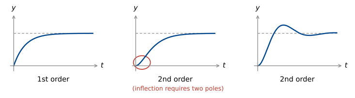
Step responses of 1^st and 2^nd order systems.

1^st order step response

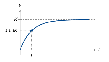
A first order model \dfrac{K}{\tau s + 1} has two parameters: the DC gain K and the time constant \tau. These can be read straight off the plot.

2^nd order step response

Underdamped

Model: \quad \dfrac{k\omega_n^2}{s^2 + 2\zeta\omega_n s + \omega_n^2}.

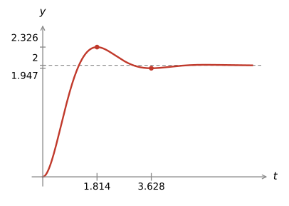
We now have three parameters to estimate.

k is the DC gain, so can be read off as the final value as for the first order system.

We can measure the damped oscillation frequency \omega_r from the time of the first peak:

\boxed{\frac{\pi}{\omega_r} = t_p} = 1.814, \quad \text{so } \omega_r = 1.732.

We can measure the percentage overshoot by

M_p = \frac{\text{peak} - k}{k} = \frac{0.326}{2} = 16.3\%.

The table in the formula sheet then gives \zeta = 0.5.

We can then find \omega_n = \dfrac{\omega_r}{\sqrt{1 - \zeta^2}} = 2\,rad/s.

Combining, we have

G(s) = \frac{8}{s^2 + 2s + 4}.

Example 2:

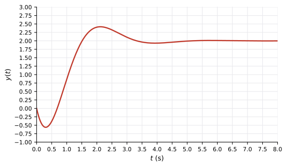
This example is not a pure second order system: it dips below zero first. This effect is caused by a right half plane zero, so we expect the form

\frac{k\omega_n^2\left(1 - \frac{s}{z}\right)}{s^2 + 2\zeta\omega_n s + \omega_n^2}.

K = 2, from the final value.

The overshoot is 0.4/2 \approx 20\%, giving \zeta = 0.45.

The peak and trough are \dfrac{\pi}{\omega_r} = 1.8 apart, so \omega_r = 1.7\,rad/s.

\omega_n = \dfrac{\omega_r}{\sqrt{1 - \zeta^2}} \approx 2\,rad/s.

This gives everything except the zero. To find the zero, we can use the initial value theorem to find the initial slope:

y'(t) \rightsquigarrow sY(s), and Y(s) = \dfrac{1}{s}G(s) \;\left(\dfrac{1}{s}\right. is the step input\left.\right).

\begin{aligned} y'(0) &= \lim_{s \to \infty} s \cdot sY(s) = \lim_{s \to \infty} sG(s) \\[8pt] &= \lim_{s \to \infty} \frac{s\,k\omega_n^2\left(1 - \frac{s}{z}\right)}{s^2 + 2\zeta\omega_n s + \omega_n^2} \\[8pt] &= -\frac{k\omega_n^2}{z}. \end{aligned}

We can measure this slope on the plot, it is -4. This gives z = 2.

Combining: \quad G(s) = \dfrac{4(2 - s)}{s^2 + 1.8s + 4}.

The true transfer function that generated the data was \dfrac{4(2 - s)}{s^2 + 2s + 4}. The error in damping is due to the table values assuming no zero.

Over-damped

Model: \quad \dfrac{k p_1 p_2}{(s + p_1)(s + p_2)}

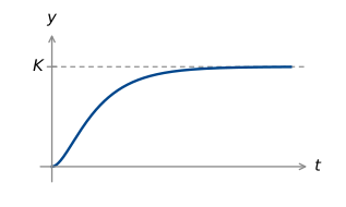
k can still be read from the final value. It is less obvious what to measure to determine p_1 & p_2 though. Better to use different test signals, like sinusoids. But first let’s look at the impulse response.

Impulse response from the step response

In principle, if we measure the step response, y(t), we can obtain the impulse response by taking the derivative:

h(t) = \frac{\mathrm{d}}{\mathrm{d}t}y(t), \quad \text{or} \quad Y(s) = \frac{1}{s}G(s).

In practice, our measurement of y(t) is not perfect, and the derivative causes issues.

Noise is generally high frequency. The derivative has Fourier transform j\omega, so the magnitude gain is \omega. This grows linearly with frequency: noise is disproportionately amplified!

We also can’t measure the true impulse response – it is a fictitious signal. But we can approximate it with pulses:

\lim_{\tau \to 0} \frac{1}{\tau}p_\tau = \delta,

so applying \dfrac{1}{\tau}p_\tau for reasonably small \tau gives a good approximation.

Frequency domain system identification

Step response methods work well for first and underdamped second order systems, and only require a single measurement. However there are some obvious limitations:

Don’t apply (or at least not accurately) with additional poles and zeros.
Single measurement creates sensitivity to measurement error.
Measurements are difficult when \zeta is close to 1 (or greater than 1).

An alternative is to take frequency domain measurements: input a sinusoid, wait for transients to settle, and measure the output sinusoid’s phase and gain.

If the input sinusoid is e^{j\omega t}, the steady state output is G(j\omega)e^{j\omega t}, so this allows us to measure |G(j\omega)| and \angle G(j\omega) experimentally. This method requires us to measure G(j\omega) at several frequencies, and interpolate between them in some way.

First, how do we measure a single frequency in a way that is robust to noise?

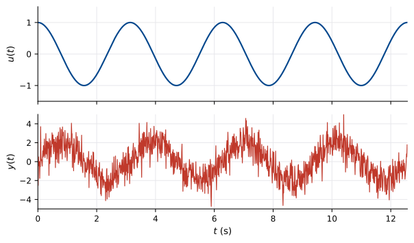
The input u(t) = \cos(2t) and the measured output y(t) of G(s) = \dfrac{8}{s^2 + 2s + 4}, with measurement noise. In steady state the noise-free output is |G(j2)|\cos\big(2t + \angle G(j2)\big) = 2\cos(2t - \pi/2).

We have already seen in week 4 how to approximate a signal as a sinusoid: this is the Fourier coefficient.

We project the signal y(t) onto the complex sinusoid \phi(t) = e^{j\omega t}:

c(y) = \langle y, \phi\rangle_P = \frac{1}{T}\int_{t_0}^{t_0 + T} y(t)e^{-j\omega t}\,\mathrm{d}t

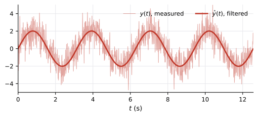
c(y) = G(j\omega), and we can write the filtered output as

\begin{aligned} \hat{y}(t) &= c(y)\phi(t) + \overline{c}(y)\overline{\phi}(t) \\[6pt] &= G(j\omega)e^{j\omega t} + \overline{G(j\omega)}e^{-j\omega t} \\[6pt] &= 2\operatorname{Re}(c)\cos\omega t - 2\operatorname{Im}(c)\sin\omega t. \end{aligned}

This method averages out any noise in the measurement.

The measured output y(t) and the filtered output \hat{y}(t), with c(y) computed over the four periods shown.

Transfer function from Bode data

The method above gets us data at a single frequency. How do we combine data at several frequencies into a model of the system? One method is to hand-fit a transfer function curve to the data on a Bode diagram.

Example:

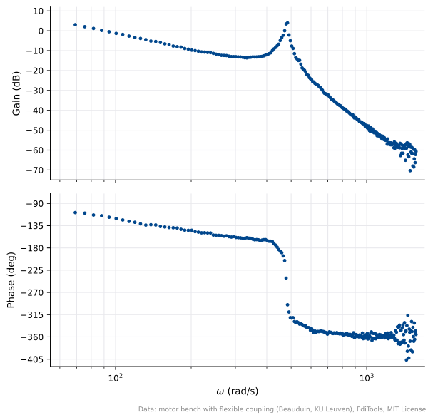
Measured data: motor current to load velocity, motor driving a load through a flexible coupling.

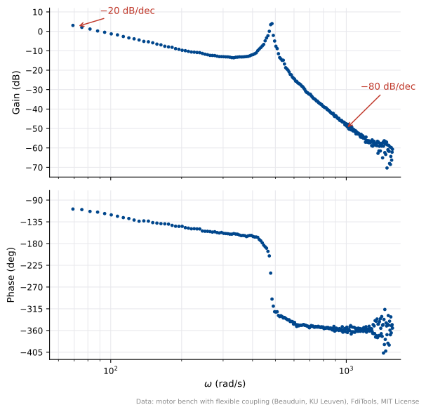
-20\,dB/dec at low frequency: integrator \dfrac{1}{s}.

-80\,dB/dec at high frequency: four poles.

Resonance at 450\,rad/s: lightly damped pair.

The resonant peak is about 15\,dB high, so \zeta \approx 0.1.

\omega_r = \omega_n\sqrt{1 - 2\zeta^2} \approx \omega_n.

We also need one extra pole. Playing around with matlab plots is one way to get it in the right spot: about 200\,rad/s.

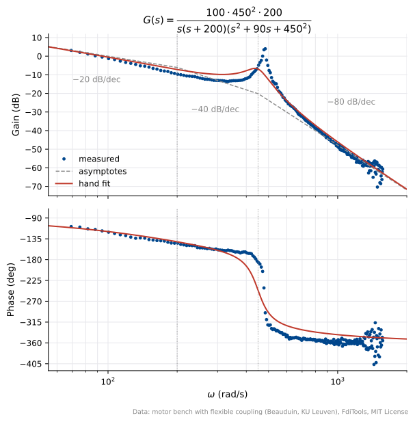
Together, this gives

G(s) = \frac{450^2 \times 200 \times k}{s(s + 200)(s^2 + 90s + 450^2)}.

To calculate k, plug in a test frequency and compare to the measured gain at that frequency.

At 70\,rad/s (lowest measurement), the (s + 200) & resonant pair have gain close to 1, so |G(j\omega)| \approx \dfrac{k}{\omega}, giving k = 98.

The hand fit, with its asymptotes, against the measured data.

Least-squares fitting a transfer function to data

We can also find the “best fit” transfer function for our frequency domain measurements, programmatically.

As this is something you’ll never do by hand, and the theory takes us a bit away from this course and into convex optimisation, I’ll illustrate this with a python notebook.

Download the notebook (motor_load_least_squares.ipynb) · Download the data (load_bode_frf.csv). Save both in the same folder.

Fitting a transfer function by least squares

Data: measured frequency response from motor current to load velocity https://github.com/HoriFujimotoLab/FdiTools/

Model structure: G(s) = \frac{b_0}{s^4 + a_3 s^3 + a_2 s^2 + a_1 s} = \frac{b_0}{D(s)}.

Unknowns: (a_3, a_2, a_1, b_0).

Hand fit: G_{\text{hand}}(s) = \dfrac{100\cdot 450^2\cdot 200}{s(s+200)(s^2+90s+450^2)}.

1. Measure \hat G(j\omega) from the data

import numpy as np
import matplotlib.pyplot as plt

d = np.loadtxt("load_bode_frf.csv", delimiter=",", skiprows=1)
w = d[:, 0]                                             # rad/s
Ghat = 10**(d[:, 2] / 20) * np.exp(1j * np.radians(d[:, 3]))
s = 1j * w
print(len(w), "frequencies from", round(w.min(), 1), "to", round(w.max(), 1), "rad/s")

240 frequencies from 69.1 to 1570.8 rad/s

2. Set up the equations

For a perfect fit, we have \hat G(j\omega_l) = b_0/D(j\omega_l) for every j\omega in the data. The division by D(j\omega) makes this nonlinear in the unknowns, so we multiply through by D(j\omega). This gives

a_3\,\hat G_l s_l^3 + a_2\,\hat G_l s_l^2 + a_1\,\hat G_l s_l - b_0 = -\hat G_l s_l^4, \qquad s_l = j\omega_l.

At each frequency, this gives a complex equation containing the data at that frequency and the unknowns (a_3, a_2, a_1, b_0). The code below stacks the real and imaginary parts of these equations into a big matrix A.

def build(Ghat, s, weight=None):
    cols = np.column_stack([Ghat * s**3, Ghat * s**2, Ghat * s, -np.ones_like(Ghat)])
    rhs = -Ghat * s**4
    if weight is not None:                      # same weight on the real and imaginary rows
        cols, rhs = cols * weight[:, None], rhs * weight
    A = np.vstack([cols.real, cols.imag])
    b = np.concatenate([rhs.real, rhs.imag])
    return A, b

A, b = build(Ghat, s)
print("A is", A.shape, "with rank", np.linalg.matrix_rank(A))

A is (480, 4) with rank 4

3. Fit by solving the normal equations

We can find the least-squares optimal curve fit by solving the normal equations (ELEC2103 Week 3):

\theta^* = (A^{\mathsf T}A)^{-1}A^{\mathsf T}b,

where \theta^* is the vector of optimal parameters (a_3, a_2, a_1, b_0). At the solution the residual A\theta^* - b is orthogonal to every column of A. We can use this to check the calculation.

theta = np.linalg.solve(A.T @ A, A.T @ b)
print("residual orthogonality, A^T(A theta - b) relative to A^T b:",
      np.abs(A.T @ (A @ theta - b)).max() / np.abs(A.T @ b).max())

def model(theta, s):
    a3, a2, a1, b0 = theta
    return b0 / (s**4 + a3 * s**3 + a2 * s**2 + a1 * s)

def describe(name, theta):
    a3, a2, a1, b0 = theta
    r = np.roots([1, a3, a2, a1])
    real = r[np.abs(r.imag) < 1e-9].real[0]
    pair = r[r.imag > 1e-9][0]
    wn, zeta = abs(pair), -pair.real / abs(pair)
    err = 20 * np.log10(np.abs(model(theta, s) / Ghat))
    print(f"{name:12s} k = {b0 / a1:6.1f}   real pole {real:7.1f}   wn = {wn:5.1f}   "
          f"zeta = {zeta:.4f}   rms gain error {np.sqrt(np.mean(err**2)):.2f} dB")

hand = np.polymul([1, 200], [1, 90, 450**2])
theta_hand = [hand[1], hand[2], hand[3], 100 * 450**2 * 200]
describe("hand fit", theta_hand)
describe("unweighted", theta)

residual orthogonality, A^T(A theta - b) relative to A^T b: 2.872977696433903e-14
hand fit     k =  100.0   real pole  -200.0   wn = 450.0   zeta = 0.1000   rms gain error 2.89 dB
unweighted   k =  107.1   real pole  -128.0   wn = 479.3   zeta = 0.0170   rms gain error 1.52 dB

4. Which frequencies dominate the error?

The equation error is

e_l = D(j\omega_l)\Big(\hat G_l - \tfrac{b_0}{D(j\omega_l)}\Big).

So the fit minimises the model error scaled by |D(j\omega_l)|, which grows like \omega^4. The highest frequencies dominate, which is where the data is noisiest.

D = s**4 + theta[0] * s**3 + theta[1] * s**2 + theta[2] * s
for x in [69, 150, 300, 480, 1000, 1500]:
    j = np.argmin(abs(w - x))
    print(f"w = {w[j]:6.1f} rad/s:  |D(jw)| = {abs(D[j]):.2e}")

w =   69.1 rad/s:  |D(jw)| = 2.26e+09
w =  150.8 rad/s:  |D(jw)| = 6.17e+09
w =  301.6 rad/s:  |D(jw)| = 1.37e+10
w =  477.5 rad/s:  |D(jw)| = 1.88e+09
w =  999.0 rad/s:  |D(jw)| = 7.73e+11
w = 1501.7 rad/s:  |D(jw)| = 4.58e+12

5. Weighted least squares

We can compensate for this effect by weighting higher frequencies less. To do this, multiply both rows in A that correspond to \omega_l by 1/|D(j\omega_l)| (taking D from the previous fit), and solve again. This normalises the frequencies so they all have close to equal weighting. Repeat until \theta^* stops changing.

theta_w = theta.copy()
for it in range(1, 5):
    D = s**4 + theta_w[0] * s**3 + theta_w[1] * s**2 + theta_w[2] * s
    Aw, bw = build(Ghat, s, weight=1 / np.abs(D))
    theta_w = np.linalg.solve(Aw.T @ Aw, Aw.T @ bw)
    describe(f"weighted {it}", theta_w)

weighted 1   k =   98.8   real pole  -132.7   wn = 479.2   zeta = 0.0165   rms gain error 1.57 dB
weighted 2   k =   98.9   real pole  -131.9   wn = 479.2   zeta = 0.0164   rms gain error 1.58 dB
weighted 3   k =   98.9   real pole  -131.9   wn = 479.2   zeta = 0.0164   rms gain error 1.58 dB
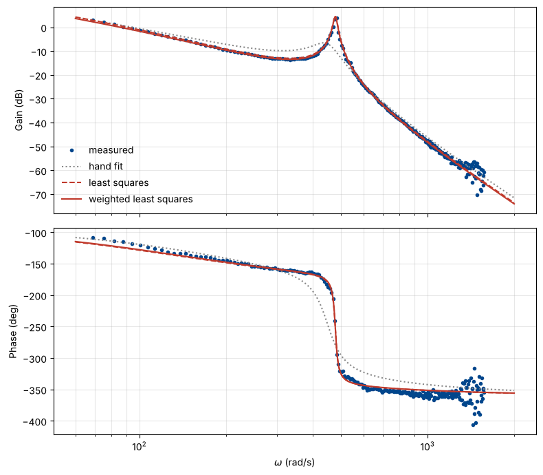
weighted 4   k =   98.9   real pole  -131.9   wn = 479.2   zeta = 0.0164   rms gain error 1.58 dB

6. Comparison of the three models

NAVY, BRICK, GREY = "#00468C", "#C0392B", "#888888"
wf = np.logspace(np.log10(60), np.log10(2000), 1500)
sf = 1j * wf

def phase(G):
    p = np.degrees(np.unwrap(np.angle(G)))
    return p - 360 * np.round((p[0] + 100) / 360)

fig, (a1, a2) = plt.subplots(2, 1, figsize=(8, 7), sharex=True)
a1.semilogx(w, 20 * np.log10(np.abs(Ghat)), "o", ms=3, color=NAVY, label="measured")
a2.semilogx(w, phase(Ghat), "o", ms=3, color=NAVY)
for th, style, lab in [(theta_hand, ":", "hand fit"), (theta, "--", "least squares"), (theta_w, "-", "weighted least squares")]:
    Gf = model(th, sf)
    col = GREY if lab == "hand fit" else BRICK
    a1.semilogx(wf, 20 * np.log10(np.abs(Gf)), style, color=col, lw=1.5, label=lab)
    a2.semilogx(wf, phase(Gf), style, color=col, lw=1.5)
a1.set_ylabel("Gain (dB)"); a2.set_ylabel("Phase (deg)"); a2.set_xlabel(r"$\omega$ (rad/s)")
a1.legend(frameon=False, loc="lower left")
for a in (a1, a2):
    a.grid(True, which="both", alpha=0.3)
plt.tight_layout()
plt.show()