Week 1 — Lecture notes
The core: exponentials, Euler’s formula and the complex plane
Other formats:
📄 PDFSignals & Systems lives at the intersection of differential equations, linear algebra, complex numbers and trigonometry.
(a) The exponential function
For z \in \mathbb{C}, define the exponential by its power series:
e^{z} := 1 + z + \frac{z^{2}}{2!} + \frac{z^{3}}{3!} + \cdots
Properties. First, e^{0} = 1 (straight from the definition) \qquad(1)
\begin{aligned} \frac{\mathrm{d}}{\mathrm{d}z}\,e^{z} &= 0 + 1 + \frac{2z}{2!} + \frac{3z^{2}}{3!} + \cdots \\[2pt] &= 1 + z + \frac{z^{2}}{2!} + \cdots \\[2pt] &= e^{z} \end{aligned} \qquad(2)
Combining the two properties:
\boxed{\,f(z) = f'(z), \qquad f(0) = 1\,}
It turns out f(z) = e^{z} is the unique solution to this differential equation, and in fact the differential equation can be used as an alternative definition.
Extension of (2). By the chain rule,
\frac{\mathrm{d}}{\mathrm{d}t}\,e^{zt} = 0 + z + \frac{2t\,z^{2}}{2!} + \frac{3t^{2}z^{3}}{3!} + \cdots = z\,e^{zt}.
(b) Euler’s formula
Let’s now represent sinusoids as complex numbers. Let
g(\theta) = \frac{\cos\theta + j\sin\theta}{e^{j\theta}} .
Then
\begin{aligned} g'(\theta) &= \big(-\sin\theta + j\cos\theta\big)e^{-j\theta} - \big(\cos\theta + j\sin\theta\big)\,j\,e^{-j\theta} \\[2pt] &= \big(-\sin\theta + j\cos\theta\big)e^{-j\theta} - \big(-\sin\theta + j\cos\theta\big)e^{-j\theta} \\[2pt] &= 0 . \end{aligned}
So g(\theta) = C (a constant):
C\,e^{j\theta} = \cos\theta + j\sin\theta .
Set \theta = 0. Then C = 1, so we have
\boxed{\,e^{j\theta} = \cos\theta + j\sin\theta\,}
What does this mean graphically? e^{j\theta} is the unit vector at angle \theta; its real part is \cos\theta and its imaginary part is \sin\theta. Advance \theta and the vector rotates, its shadow tracing a sinusoid.
In particular: \;e^{j\pi/2} = j, \qquad e^{j\pi} = -1.
Manipulating sinusoids using complex numbers
Why use complex numbers to represent sinusoids? Because it makes the algebra easier. For example,
x_1(t) = 3\cos\omega t, \qquad x_2(t) = 4\cos\!\big(\omega t + \tfrac{\pi}{2}\big), \qquad x_1(t) + x_2(t) = \;?
The direct way uses the identity \cos(\theta + \tfrac{\pi}{2}) = -\sin\theta, so x_2(t) = -4\sin\omega t, giving
3\cos\omega t - 4\sin\omega t \;\equiv\; A\cos(\omega t + \varphi) \quad\longrightarrow\quad \text{match coefficients} \dots
With complex numbers:
\begin{aligned} x_1(t) &= \operatorname{Re}\!\big(3\,e^{j\omega t}\big) \\[2pt] x_2(t) &= \operatorname{Re}\!\big(4\,e^{\,j\omega t + j\pi/2}\big) = \operatorname{Re}\!\big(4\,e^{j\pi/2}\,e^{j\omega t}\big) = \operatorname{Re}\!\big(4j\,e^{j\omega t}\big) \\[2pt] x_1(t) + x_2(t) &= \operatorname{Re}\!\big(3\,e^{j\omega t} + 4j\,e^{j\omega t}\big) \\[2pt] &= \operatorname{Re}\!\big((3 + 4j)\,e^{j\omega t}\big) \\[2pt] &= \operatorname{Re}\!\big(5\,e^{j0.927}\,e^{j\omega t}\big) = 5\cos(\omega t + 0.927). \end{aligned}
The triangle 3 + 4j = 5\angle 53.1^{\circ} rotates.
(c) Euler’s formula & differential equations
Another differential equation:
\frac{\mathrm{d}}{\mathrm{d}t}\,x(t) = j\,x(t) \qquad(3)
We’ve already seen \dfrac{\mathrm{d}}{\mathrm{d}t}e^{zt} = z\,e^{zt}. Set z = j:
\frac{\mathrm{d}}{\mathrm{d}t}\,e^{jt} = j\,e^{jt}.
This solves (3). What does it look like in \mathbb{C}, and what does the real part look like? What about other choices of z?
z = -1:\quad \frac{\mathrm{d}}{\mathrm{d}t}\,e^{-t} = -e^{-t}. \qquad\text{No imaginary component.}
z = -1 + j:\quad \frac{\mathrm{d}}{\mathrm{d}t}\,e^{(-1+j)t} = (-1+j)\,e^{(-1+j)t}.
The widget below plots the trajectory of e^{zt} for several values of z.
The position of z determines the behaviour: oscillations, decay, growth.
(d) What has this got to do with electrical engineering?
Example: an RLC circuit (the system) with a sinusoidal voltage input (the signal).
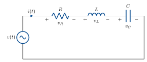
KVL around the loop:
v(t) = v_R + v_L + v_C
v(t) = R\,i(t) + L\,\frac{\mathrm{d}i(t)}{\mathrm{d}t} + \frac{1}{C}\!\int_{-\infty}^{t}\! i(\tau)\,\mathrm{d}\tau \qquad(4)
with the lower limit taken to -\infty for the steady-state response. Let v(t) = V\cos\omega t = \operatorname{Re}(V e^{j\omega t}) and look for a current of the same form, i(t) = \operatorname{Re}(I e^{j\omega t}).
Substitute in (4):
\begin{aligned} V e^{j\omega t} &= R I e^{j\omega t} + L\frac{\mathrm{d}}{\mathrm{d}t}I e^{j\omega t} + \frac{1}{C}\!\int\! I e^{j\omega\tau}\,\mathrm{d}\tau \\[2pt] &= R I e^{j\omega t} + j\omega L\, I e^{j\omega t} + \frac{I}{j\omega C}\,e^{j\omega t} + \frac{K}{C}, \end{aligned} where K is a constant of integration. Matching coefficients of e^{j\omega t}, we find K = 0 (K represents a residual charge on the capacitor, which a sinuosoidal voltage is not able to maintain at steady state).
Divide through by e^{j\omega t} (never zero):
V = I\underbrace{\Big(R + j\omega L + \tfrac{1}{j\omega C}\Big)}_{\text{impedance } Z(j\omega)} \qquad\Longrightarrow\qquad I = \frac{V}{Z}.
Suppose R = 30\,\Omega and \omega L - \tfrac{1}{\omega C} = 40\,\Omega. Then
Z = 30 + 40j = 50\,e^{j0.927}, \qquad I = \frac{V}{50\,e^{j0.927}},
i(t) = \operatorname{Re}(I e^{j\omega t}) = \frac{V}{50}\cos(\omega t - 0.927).
The widget below plots input and output sinusoids for several values of the reactance Z. For some values, the output lags the input, while for others, the output leads.
The RLC circuit maps a sinusoid to a sinusoid with the same frequency. This is the foundation of the rest of the course.