ELEC2302/9302: Signals and Systems
Week 1: Introduction · Semester 2, 2026
Signals and systems
A signal is a function that carries information: a voltage on a wire, the price of a barrel of oil, the brightness of a pixel, the pressure of the air in this room.
A system takes a signal in and puts a signal out: an amplifier, a filter, a circuit, a trading algorithm, a lens.
Course outline
Foundations Weeks 1–3
- Signals, systems, differential equations, Euler’s formula
- Signals as vectors, systems as maps
- LTI systems, impulse response, convolution
Frequency domain Weeks 4–6
- Periodic signals and the Fourier series
- Aperiodic signals and the Fourier transform
- Frequency response
Systems and Laplace Weeks 7–9
- System response and stability
- The Laplace transform
- System analysis with the Laplace transform
Applications Weeks 10–13
- Filter design
- Signal modulation
- System identification
- Advanced topics
Everything is a different way of looking at the same object: a linear, time-invariant system. Both mathematically elegant and extremely useful: the core of electrical engineering.
Classes
Lecture — two hours a week, Monday 15:00-17:00. Typeset notes go up a couple of days before.
Tutorials — two hours, Weeks 2–13. Ten tutorials (two weeks are labs). This is where the quizzes happen.
Labs — two practicals on the TIMS hardware, in Weeks 6 and 8 for half the tutorial groups and Weeks 7 and 9 for the other half. Attendance is mandatory.
Times, rooms and which lab weeks apply to you are on your timetable. There is no tutorial in Week 1.
Course materials
Lectures, tutorials and lab instructions will be posted on the course website: tchaffey.com/elec2302.
Anything to do with assessments: Canvas.
Discussion: Ed.
There is a prereq revision quiz available on Canvas.
Assessment
| Tutorial prework |
4% |
Weekly, from Week 2 |
| Quiz 1 |
10% |
Week 4 tutorial + two more attempts |
| Quiz 2 |
15% |
Week 8 or 9 tutorial + two more attempts |
| Quiz 3 |
15% |
Week 12 tutorial + one more attempt |
| Lab 1 milestones |
3% |
In your lab |
| Lab 2 milestones |
3% |
In your lab |
| Final exam |
50% |
Formal exam period |
| Bonus extension quizzes |
+2.5% each |
after quiz 2 and quiz 3 if you have an HD |
Prework
Prework is marked for a genuine attempt, not for being right: 0.5% each, capped at 4%. That is eight of the ten tutorials, so you can miss two without losing anything.
Prework must be handwritten. Take a photo before you hand it in.
Quizzes
Three quizzes, each 30 minutes, in your tutorial.
You need 70% in each quiz to pass the unit.
- More than one attempt at every quiz: three at Quizzes 1 and 2, two at Quiz 3.
- Each attempt is in a later tutorial, and your best mark is the one that counts.
- The questions change between attempts but test the same material. You cannot look up last week’s answers.
The bar is high because you get more than one go at it. Needing a second attempt is normal!
- An HD in Quiz 2 or Quiz 3 unlocks a Bonus Quiz, where you can earn up to 2.5% top up marks (per quiz).
When your quizzes happen
Quizzes run in tutorials. Your attempts are in your next tutorials, so if you have a lab, your quiz will be the week after.
If your labs are Weeks 6 and 8
- Quiz 1 — Weeks 4, 5, 7
- Quiz 2 — Weeks 9, 10, 11
- Quiz 3 — Weeks 12, 13
If your labs are Weeks 7 and 9
- Quiz 1 — Weeks 4, 5, 6
- Quiz 2 — Weeks 8, 10, 11
- Quiz 3 — Weeks 12, 13
Some groups sit a quiz a week before others. Different groups get different versions, and every group gets the same number of attempts, so nobody is advantaged by the timetable. Your weeks are on your timetable.
What the quizzes look like
On Canvas, locked-down browser
- Short numeric answers — calculations
- Multiple choice — concepts and reasoning
You get a formula sheet and can use a calculator. The formula sheet is on the course website tchaffey.com/elec2302.
Tutorials and exam
In the tutorials, you will work through practice problems. These are designed to develop and extend the concepts in the lectures and give you practical experience analysing signals and systems.
The exam will be closely modelled on the tutorial problems.
Where to find help
Me — straight after this lecture, and in office hours (email me to make an appointment: thomas.chaffey@sydney.edu.au).
Your tutors — in tutorials and labs. They see your work every week and they are the fastest route to an answer.
Ed Discussion — ask and answer! Teaching staff will attempt to answer unanswered questions within a day.
Canvas — notes, prework, quiz details, everything administrative.
Expectations
What you can expect of us
- Quiz and prework marks within one week
- Answering emails and Ed posts within two working days (aiming for one)
- Answering questions during tutorials, after lecture
- Clear guidelines for quizzes and the exam
What we expect of you
- About 6hrs independent study per week, as well as tutorial and lecture
- Attend your tutorials and labs
- Attempt prework before the tutorial
- Attend or read lecture before the tutorial
- Complete the tutorial problems after the tutorial
- Ask questions
- Have fun!
Pass/credit standard: able perform calculations and system analysis to a sufficient standard for third year courses.
D/HD standard: understand the underlying concepts and structures, perform analysis beyond the example problems.
What is this course about?
Signals and systems
A signal is a function that carries information: a voltage on a wire, the price of a barrel of oil, the brightness of a pixel, the pressure of the air in this room.
A system takes a signal in and puts a signal out: an amplifier, a filter, a circuit, a trading algorithm, a lens.
Example 1: seeing through cloud
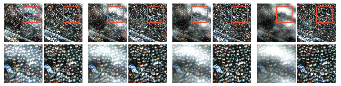
Thin cloud removal from satellite imagery. Left of each pair: the observed scene. Right: the recovered surface. The cloud is separated from the ground by filtering.
Lei, M., Li, H., Xu, L., & Shen, H. (2025). Diffusion generation with homomorphic filtering for remote sensing thin cloud removal. Geo-Spatial Information Science, 1–14.
Example 2: the price of oil
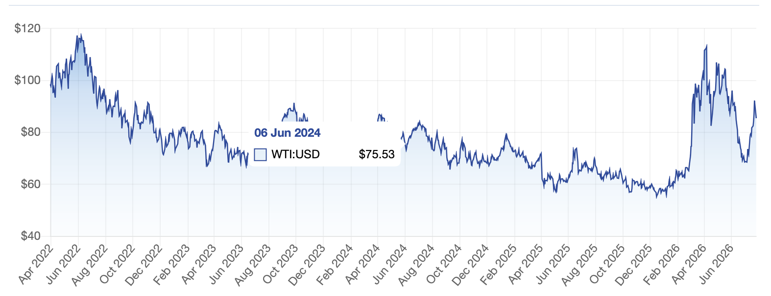
West Texas Intermediate crude, April 2022 to July 2026. One price per trading day.
Example 3: algorithmic trading
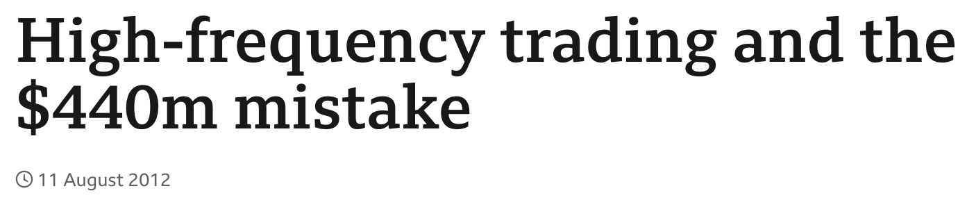
Knight Capital, 1 August 2012. A rogue trading system ran for 45 minutes and lost US$440 million (about $10 million a minute).
Headline: BBC News, 11 August 2012.
Example 4: filtering sound
A 100 Hz square wave through a resonant low-pass filter. Move the cutoff and listen to the harmonics disappear one at a time.
Example 5: positioning a silicon wafer
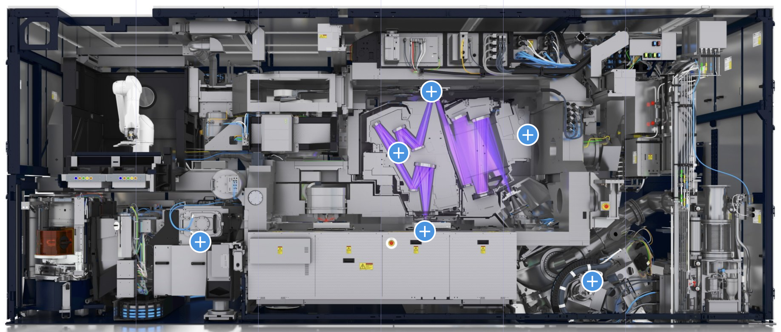
A lithography machine prints circuit patterns onto a wafer that is being moved underneath the optics. The stage has to follow its trajectory to within nanometres while accelerating hard to maximise throughput.
Signals — the measured stage position, and the torque commanded to the motors. System — the wafer stage being positioned.
Cutaway of an extreme-ultraviolet lithography system. Image: ASML.
Example 6: the FFT is everywhere!
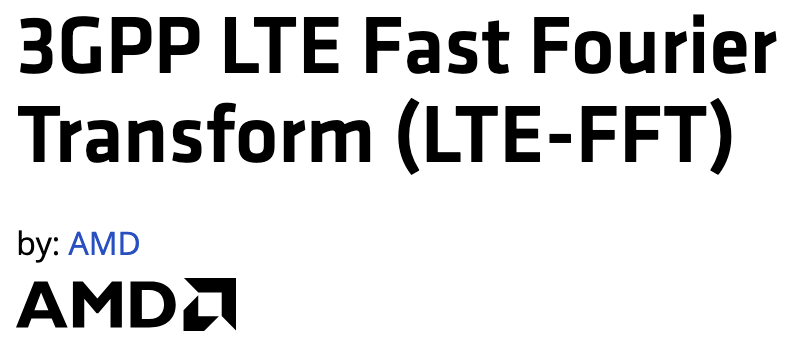
Wi-Fi and 5G rely on specialised chips that compute the Fast Fourier Transform of every incoming and outgoing signal. In Wi-Fi, a 64-point transform runs every 4 µs: a quarter of a million transforms a second.
LTE-FFT IP core, AMD. Waveform defined in IEEE Std 802.11a-1999 §17.3.5.9 and 3GPP TS 36.211 §6.12.
Example 7: convolution for machine learning
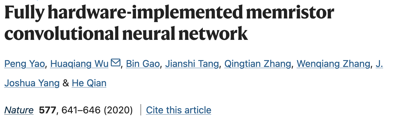
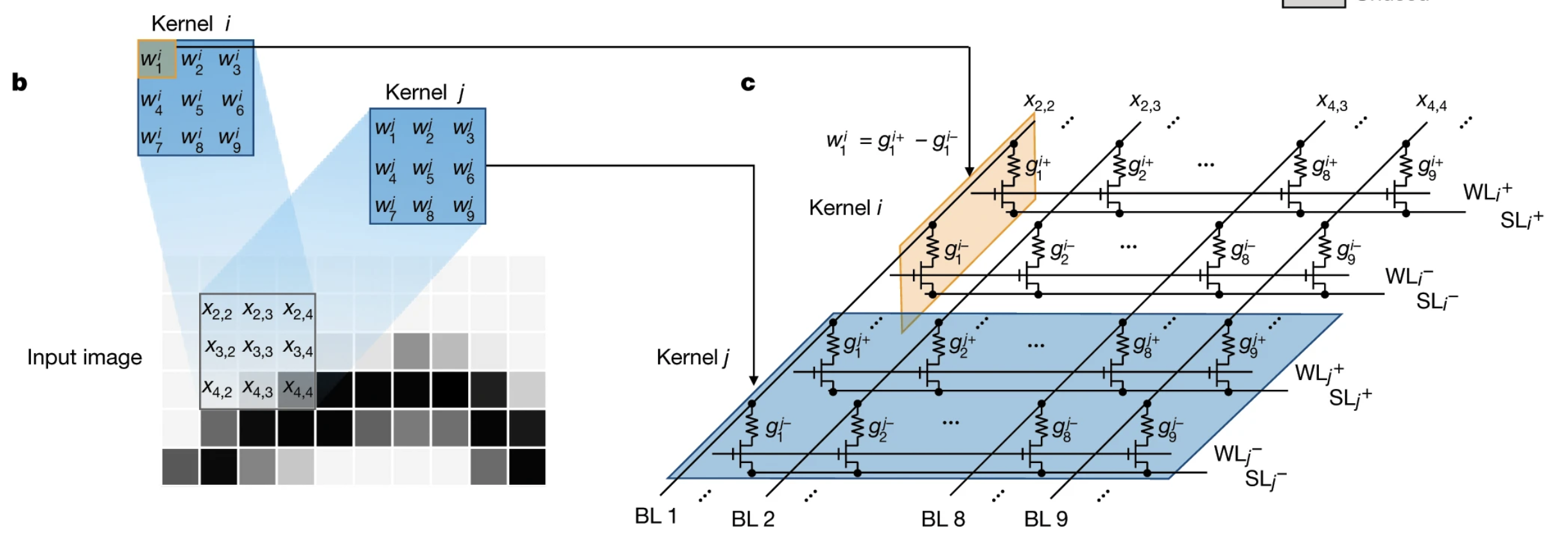
A neural network built from memristor crossbars. The convolution (an operation we will learn in Week 3) is the foundation of Convolutional Neural Networks. The figure shows an experimental design for computing the convolution in the array itself, by Ohm’s law and Kirchhoff’s current law. This is two orders of magnitude more energy-efficient than a GPU.
Yao, P., Wu, H., Gao, B., Tang, J., Zhang, Q., Zhang, W., Yang, J. J., & Qian, H. (2020). Fully hardware-implemented memristor convolutional neural network. Nature, 577, 641–646.
Types of signals
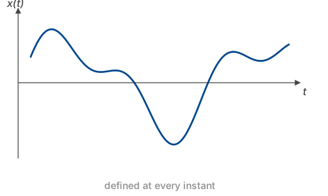
A continuous-time signal has a value at every instant: the air pressure at your ear, the voltage across a capacitor, the current in a circuit.
x(t), \qquad t \in \mathbb{R}
![]()
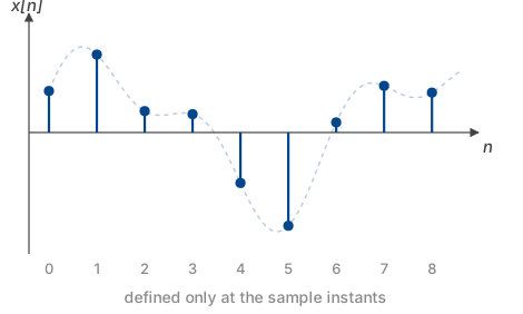
A discrete-time signal has a value only at particular instants: the closing price each day, the samples in an audio file, the pixels in an image.
x[n], \qquad n \in \mathbb{Z}
![]()
Of the examples so far: the sound and the wafer stage were continuous, the oil price and the radio samples were discrete, and the satellite image was discrete in two spatial dimensions rather than in time.
What will we learn in this course?
Continuous-time signals and linear, time-invariant systems.
Two views of the same system, and the translation between them:
- Time domain — differential equations, impulse response, convolution.
- Frequency domain — Fourier series, Fourier transform, Laplace transform.
Linear and time-invariant are strong assumptions. They are also the assumptions that make the problem solvable, and they hold well enough to have built most of the twentieth century.
Why is this useful?
These are the foundations of:
Systems
- Control
- Stability analysis
- System identification
Communications
- Modulation
- Filtering
- Sampling
Devices
- Analogue electronics
- Photonics
- Power systems
Computation
- Signal processing
- Convolutional neural networks
- Imaging
Where we start
Signals and systems sits at the intersection of differential equations, linear algebra, complex numbers and trigonometry.
Rest of today’s lecture: the exponential function, Euler’s formula, and the complex plane.
Adding sinusoids
3\,e^{j\omega t} + 4j\,e^{j\omega t} = 5\,e^{j0.927}e^{j\omega t}
Sinusoid in, sinusoid out
V = I\Big(R + j\omega L + \tfrac{1}{j\omega C}\Big) = I\,Z(j\omega)
\qquad\Longrightarrow\qquad I = \frac{V}{Z}