Week 11 — Lecture notes

Motivation: wireless communication

Example 1

When we transmit audio over a wire, we simply transmit the signal (with some amplification and filtering):

What about when we transmit wirelessly?

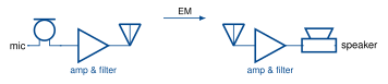
Audio over the air, with an antenna at each end.

The length of the antenna has to be proportional to the wavelength of the signal.

Q: telephone audio contains frequencies from 200–3000\,Hz. What order of magnitude should the antenna length be? \; mm, cm, m, km, \geq 100\,km?

Q: what frequencies of EM are matched to a 10\,cm antenna?

We need a way to shift the signal we want to transmit to the frequencies we can transmit.

Example 2: we saw in the week 5 lecture that there is a tradeoff in radar resolution and bandwidth. A narrow pulse (\tau\,s) corresponds to a wider spectrum. For Kurnell, the pulse width is 1.8\,\mus. The first null of the spectrum is \dfrac{2\pi}{\tau} = 3.5\times10^{6}\,rad/s.

Week 5: the width-\tau pulse and its spectrum (widget)

The spectrum of the pulse is centred at zero. However, if you look up the spectrum assignment in the ACMA (Australian Communications & Media Authority) Licence register, the allocated bandwidth is centred at 5.625\,GHz.

How do we shift the spectrum there?

This is the function of modulation: shifting the frequency spectrum. There is a zoo of modulation techniques.

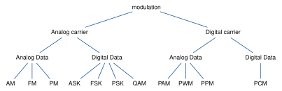
Modulation techniques, grouped by carrier and by data.

In this lecture, we’ll look at the three methods on the left, AM, FM and PM. They are the basis for many of the other methods.

Amplitude Modulation

This method is already hiding in plain sight on the formula sheet!

u(t)\cos(\omega_0 t) \;\overset{\text{F.T.}}{\rightsquigarrow}\; \tfrac{1}{2}U\big(j(\omega-\omega_0)\big) + \tfrac{1}{2}U\big(j(\omega+\omega_0)\big).

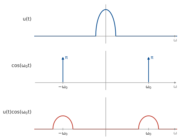
Spectra of u(t), \cos(\omega_0 t) and u(t)\cos(\omega_0 t).

This is called Amplitude Modulation (AM). \cos(\omega_0 t) is called the carrier.

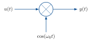
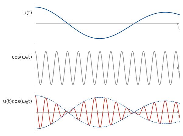
The message u(t), the carrier \cos(\omega_0 t) and the product u(t)\cos(\omega_0 t), with \pm u(t) dashed.

The amplitude of the carrier is modulated by the signal.

Demodulation

How do we recover the signal at the receiver?

If we multiply by the carrier again, we get

\begin{aligned} z(t) &= y(t)\cos(\omega_0 t) \\[6pt] &= u(t)\big(\cos(\omega_0 t)\big)^2 \\[6pt] &= \tfrac{1}{2}u(t)\big(1 + \cos(2\omega_0 t)\big) \end{aligned}

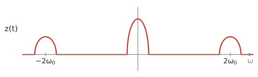
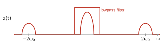
Spectrum of z(t): \tfrac{1}{2}U at the origin, \tfrac{1}{4}U at \pm 2\omega_0.

We can then lowpass filter to get back u(t).

Spectrum of z(t), with the lowpass filter.

Frequency division multiplexing

What if we want to transmit multiple signals simultaneously? Use separate carrier frequencies: Frequency Division Multiplexing.

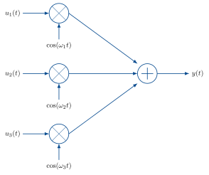
Three signals on three carriers, summed.

How do we demodulate this sum? The receiver can choose which signal to demodulate by multiplying by the corresponding carrier.

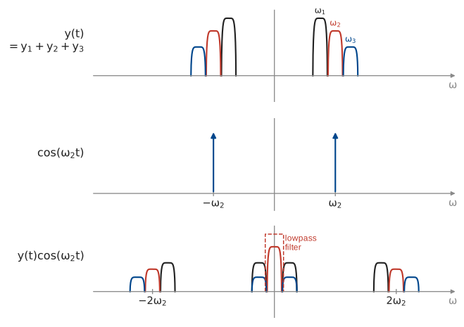
Demodulating with \cos(\omega_2 t). Black, red and blue are the channels on \omega_1, \omega_2 and \omega_3.

If instead we multiply by \cos(\omega_1 t):

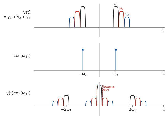
This is how the radio station selector on an AM radio works.

Frequency modulation

There are two other common ways to embed an analog signal in an analog carrier: frequency modulation and phase modulation.

\begin{aligned} &\text{Amplitude modulation:} && y(t) = u(t)\cos(\omega_c t) \\[6pt] &\text{Frequency modulation:} && y(t) = \cos\!\Big(\omega_c t + k\int_{-\infty}^{t} u(\tau)\,\mathrm{d}\tau\Big) \\[6pt] &\text{Phase modulation:} && y(t) = \cos\big(\omega_c t + k u(t)\big) \end{aligned}

For a sinusoid with variable frequency, y(t) = \cos\big(\omega(t)\,t\big), we define the instantaneous frequency to be

\omega_i = \frac{\mathrm{d}}{\mathrm{d}t}\big(\omega(t)\,t\big).

For a sinusoid with constant frequency, \cos(\omega t), this is just the usual frequency: \;\dfrac{\mathrm{d}}{\mathrm{d}t}\,\omega t = \omega.

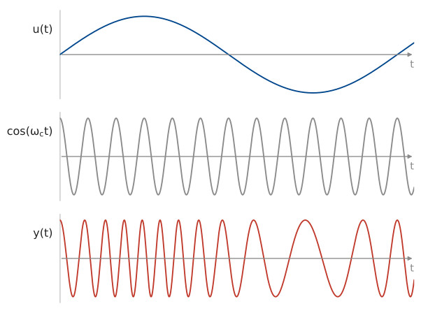
For an FM signal, the instantaneous frequency is

\begin{aligned} &\frac{\mathrm{d}}{\mathrm{d}t}\Big(\omega_c t + k\int_{-\infty}^{t} u(\tau)\,\mathrm{d}\tau\Big) \\[8pt] &= \omega_c + k\,\frac{\mathrm{d}}{\mathrm{d}t}\int_{-\infty}^{t} u(\tau)\,\mathrm{d}\tau \\[8pt] &= \omega_c + k u(t). \end{aligned}

So the signal u(t) modulates the instantaneous frequency of the carrier.

The message u(t), the carrier \cos(\omega_c t) and the FM signal y(t).

What is the bandwidth of FM?

y(t) = \cos\!\Big(\omega_c t + k\int_{-\infty}^{t} u(\tau)\,\mathrm{d}\tau\Big)

If we let k \to 0, is the spectrum concentrated at \omega_c?

y(t) = \cos(\omega_c t)\cos\!\Big(k\int_{-\infty}^{t} u(\tau)\,\mathrm{d}\tau\Big) - \sin(\omega_c t)\sin\!\Big(k\int_{-\infty}^{t} u(\tau)\,\mathrm{d}\tau\Big)

As k \longrightarrow 0:

\begin{aligned} \cos\!\Big(k\int_{-\infty}^{t} u(\tau)\,\mathrm{d}\tau\Big) &\longrightarrow 1 \\[8pt] \sin\!\Big(k\int_{-\infty}^{t} u(\tau)\,\mathrm{d}\tau\Big) &\longrightarrow k\int_{-\infty}^{t} u(\tau)\,\mathrm{d}\tau. \end{aligned}

So

y(t) \approx \cos(\omega_c t) \underbrace{- \sin(\omega_c t)\,k\int_{-\infty}^{t} u(\tau)\,\mathrm{d}\tau}_{\substack{\text{same bandwidth as AM} \\ \text{– the bandwidth of } \int u(\tau)\,\mathrm{d}\tau}}.

What is the bandwidth for large k?

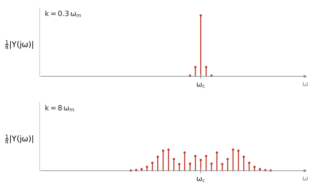
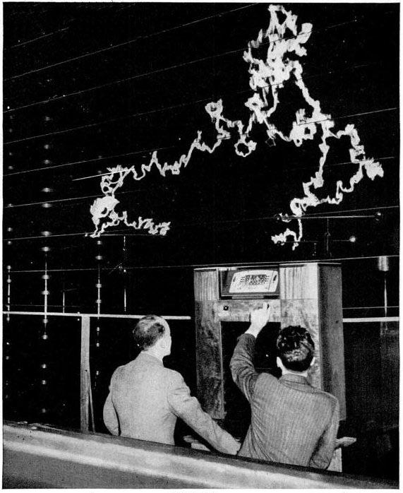
Spectrum of y(t) for the single-tone message u(t) = \cos(\omega_m t), positive frequencies only. For this message y(t) = \cos\big(\omega_c t + \tfrac{k}{\omega_m}\sin(\omega_m t)\big), whose transform has impulses of weight \pi J_n(k/\omega_m) at \omega_c + n\omega_m. Top: k = 0.3\,\omega_m. Bottom: k = 8\,\omega_m.

So FM spreads the signal all over the spectrum. This makes it very robust to noise.

A 1940s demonstration of FM’s robustness to noise. It reproduces a broadcast despite the 1 MV arc in the background. Source: Wikipedia.

Phase modulation

PM is closely related to FM, but instead of modulating the instantaneous frequency, we modulate phase.

y(t) = \cos\big(\omega_c t + u(t)\big).

This is the same as FM with signal u'(t): calculating the instantaneous frequency of the PM signal, we have

\frac{\mathrm{d}}{\mathrm{d}t}\big(\omega_c t + u(t)\big) = \omega_c + u'(t).

Example: FM Stereo Multiplexing

How do we transmit both left and right audio channels over FM?

We transmit a composite signal that uses AM to carry both channels: \qquad \omega_p = 2\pi\cdot 19\,\text{kHz}.

u(t) = \underbrace{\big(L(t) + R(t)\big)}_{0\text{–}15\,\text{kHz}} + \underbrace{A_p\cos(\omega_p t)}_{19\,\text{kHz}} + \underbrace{\big(L(t) - R(t)\big)\cos(2\omega_p t)}_{23\text{–}53\,\text{kHz}}.

How do we recover L(t) & R(t) at the receiver?

There are 4 steps.

1. Sum recovery.

2. Carrier recovery.

G is a narrow bandpass filter at 19\,kHz.

Squaring the output gives

A_p^2\,|G(j\omega_p)|^2\cos(\omega_p t + \theta)^2 = \tfrac{1}{2}A_p^2\,|G(j\omega_p)|^2\big(1 + \cos(2\omega_p t + 2\theta)\big).

Pass this through a narrow bandpass at 2\omega_p = 2\pi\cdot 38\,\text{kHz} to remove the constant, and normalise amplitude to get \cos(2\omega_p t + 2\theta).

3. Difference recovery.

Multiply u(t) by \cos(2\omega_p t + 2\theta) to get

\begin{aligned} &(L+R)\cos(2\omega_p t + 2\theta) + \colorbox{lightblue}{$A_p\cos(\omega_p t)\cos(2\omega_p t + 2\theta)$} \\[6pt] &\quad + \colorbox{peachpuff}{$(L-R)\cos(2\omega_p t)\cos(2\omega_p t + 2\theta)$} \end{aligned}

Simplify the 2^nd & 3^rd terms using \cos a\cos b = \tfrac{1}{2}\big(\cos(a-b) + \cos(a+b)\big).

\colorbox{lightblue}{$A_p\cos(\omega_p t)\cos(2\omega_p t + 2\theta)$} = \tfrac{1}{2}A_p\cos(\omega_p t + 2\theta) + \tfrac{1}{2}A_p\cos(3\omega_p t + 2\theta)

\colorbox{peachpuff}{$(L-R)\cos(2\omega_p t)\cos(2\omega_p t + 2\theta)$} = \tfrac{1}{2}(L-R)\cos(2\theta) + \tfrac{1}{2}(L-R)\cos(4\omega_p t + 2\theta).

Putting all the terms together, we get

\begin{aligned} &\underbrace{\tfrac{1}{2}(L-R)\cos(2\theta)}_{0\text{–}15\,\text{kHz}} + \underbrace{\tfrac{1}{2}A_p\cos(\omega_p t + 2\theta)}_{19\,\text{kHz}} + \underbrace{(L+R)\cos(2\omega_p t + 2\theta)}_{23\text{–}53\,\text{kHz}} \\[10pt] &+ \underbrace{\tfrac{1}{2}A_p\cos(3\omega_p t + 2\theta)}_{57\,\text{kHz}} + \underbrace{\tfrac{1}{2}(L-R)\cos(4\omega_p t + 2\theta)}_{61\text{–}91\,\text{kHz}}. \end{aligned}

Passing this through a lowpass filter with cutoff 15\,kHz, we get \tfrac{1}{2}(L-R)\cos(2\theta).

\theta is the filter phase, which is part of the design, so we can divide it off to recover L-R.

4. Channel recovery.

Add: \;L-R + L+R\; to get 2L.

Subtract: \;L-R - (L+R) = -2R.