Week 10 — Lecture notes

Filter design

Other formats:

Lecture outline

Intro, motivation
Ideal filters: lowpass, highpass, bandpass, bandstop, allpass.
Realisable filter specifications
1^st & 2^nd order filters
Audio example.
Building bandpass and bandstop filters.
Butterworth filters.
Design example 2.

“Filtering” a signal means removing unwanted parts of its frequency spectrum. For example:

Ferrite beads on cables remove radio frequency interference
Ripple filters on power supplies smooth converted AC signals
Suspension filters out road noise/bumps.
Rumble filters reject slow oscillations caused by warped vinyl records.
Earthquake vibration suppression that we saw last week
Anti-aliasing filters before converting analogue to digital.
And many more. Any piece of electronics is full of filters.

This lecture will give an introduction to how we design filters from given specifications. This is a broad topic, there is much more to learn!

Ideal filters

An ideal filter has two characteristics:

Perfect transmission (no distortion) of the signals we want (the “passband”).
Perfect rejection of the signals we don’t want (the “stopband”).

There are four ideal filter types:

Ideal lowpass: gain 1 below omega_c, 0 above.

Ideal highpass: gain 0 below omega_c, 1 above.

Ideal bandpass: gain 1 between omega_1 and omega_2, 0 elsewhere.

Ideal bandstop: gain 0 between omega_1 and omega_2, 1 elsewhere.

Ideal allpass (buffer): gain 1 at all frequencies.

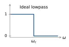
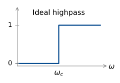
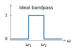
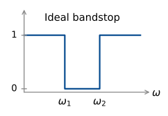
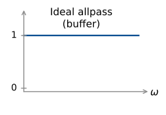
Can we build an ideal filter?

Let’s look more closely at the ideal lowpass filter. If we consider negative frequencies as well, we have

\begin{aligned} G(j\omega) &= \begin{cases} 1, & \lvert\omega\rvert < \omega_c \\ 0, & \lvert\omega\rvert > \omega_c. \end{cases} \\[10pt] &= p_{2\omega_c}(\omega) \end{aligned}

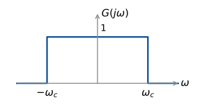
G(j omega) equal to 1 between minus omega_c and omega_c, 0 outside.

We can find the impulse response of this filter by finding the inverse Fourier transform in our table of transforms:

\begin{aligned} g(t) &= \frac{\sin(\omega_c t)}{\pi t} \\[10pt] &= \frac{\omega_c}{\pi}\,\frac{\sin(\pi T)}{\pi T} \qquad \text{where } T = \frac{\omega_c t}{\pi}. \\[10pt] &= \frac{\omega_c}{\pi}\operatorname{sinc}(T) = \frac{\omega_c}{\pi}\operatorname{sinc}\!\left(\frac{\omega_c t}{\pi}\right). \end{aligned}

\begin{aligned} \pi T &= \omega_c t \\[4pt] T &= \frac{\omega_c t}{\pi}, \qquad t = \frac{\pi T}{\omega_c} \end{aligned}

\text{So } \frac{1}{\pi t} = \frac{\omega_c}{\pi^2 T} = \frac{\omega_c}{\pi}\,\frac{1}{\pi T}

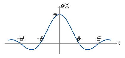
The impulse response g(t), a sinc centred on t = 0 with peak omega_c over pi, nonzero for negative and positive time.

The impulse response goes backwards in time as well as forwards! No surprise, this can’t be built (unless you record the whole signal first then filter it).

Realisable filter specifications

So in practice, we need to compromise on the ideal filter characteristics of perfect transmission of the passband and perfect rejection of the stopband. A real low pass filter has an amplitude response in an allowable region:

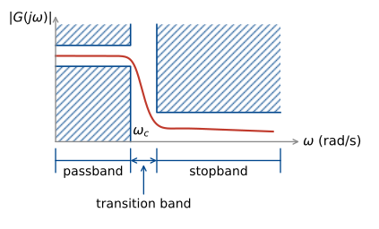
Allowable region for a lowpass gain: hatched forbidden regions above and below the passband up to omega_c, and above the stopband level beyond the transition band. The passband, transition band and stopband are marked on the frequency axis.

The width of the passband is also known as the bandwidth for a low pass filter. Its precise definition depends on the specification, but commonly it is the frequency where the gain first drops below -3 dB.

We have already seen many low pass filters in this course:

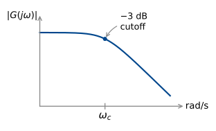
Gain of a first order lowpass: flat, then falling, with the minus 3 dB cutoff at omega_c.

\frac{1}{j\omega + \omega_c}

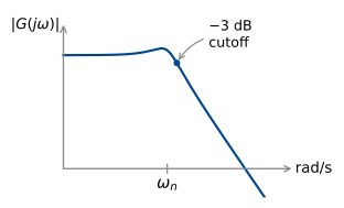
Gain of a second order lowpass: flat, a small peak near omega_n, the minus 3 dB cutoff just above it, then falling.

\frac{\omega_n^2}{(j\omega)^2 + 2\omega_n\zeta j\omega + \omega_n^2}

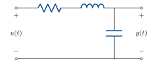
Series RLC circuit with input u(t) and output y(t) across the capacitor.

We’ve also seen high pass filters (although they have infinite gain at high frequency, which of course can’t actually be built).

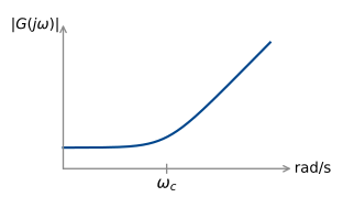
Gain of j omega plus omega_c: flat, then rising after omega_c.

j\omega + \omega_c

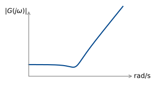
Gain of a complex zero pair: flat, a dip, then rising.

\frac{(j\omega)^2 + 2\omega_n\zeta j\omega + \omega_n^2}{\omega_n^2}

Design example 1: RIAA phono equalisation

A turntable converts a mechanical signal cut into a vinyl record into an electrical signal using a stylus and cartridge:

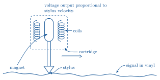
Moving magnet cartridge: a magnet on the stylus cantilever sits between two coils inside the cartridge. The stylus tip follows the groove, the signal in the vinyl, as the record moves.

(A moving magnet style cartridge).

Low frequencies move slower, so large grooves must be cut to achieve the same stylus velocity. This reduces the length of signal that can be represented on the vinyl. For this reason, it is standard to filter the signal before cutting the vinyl, to reduce the amplitude at low frequencies. At playback, this filtering is reversed, by a phono stage. The most common specification is RIAA (Recording Industry Association of America). This specification also boosts high frequencies at recording, which are then attenuated at playback. This means surface noise (pops, clicks) are also attenuated.

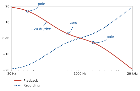
RIAA playback curve falling from about +19 dB at 20 Hz to about −20 dB at 20 kHz through 0 dB at 1 kHz, with the recording curve its mirror image. Poles marked at 50 Hz and 2122 Hz and a zero at 500 Hz on the playback curve, with a −20 dB per decade slope marked.

The curve is specified by three first order break frequencies:

\begin{aligned} f_1 &= 50.05\ \text{Hz} &&= 314.5\ \text{rad/s} &&(\text{pole}) \\[4pt] f_2 &= 500.5\ \text{Hz} &&= 3145\ \text{rad/s} &&(\text{zero}) \\[4pt] f_3 &= 2122\ \text{Hz} &&= 13333\ \text{rad/s} &&(\text{pole}). \end{aligned}

It is customary to normalise by setting the gain to 0 dB at 1\ \text{kHz} = 6283\ \text{rad/s}.

What is the transfer function of this filter?

We can read the poles and zeros directly from the specification:

G(j\omega) = \frac{(j\omega + 3145)\,k}{(j\omega + 314.5)(j\omega + 13333)}

To find the gain k, we substitute \omega = 6283 and find \lvert G(j\omega)\rvert. First, find the gain of each component:

\lvert(j\omega + p)\rvert = \sqrt{\omega^2 + p^2}

\left\{ \begin{aligned} &\text{pole at } 314.5\text{:} &\quad 6291.0 &= p_1 \\[4pt] &\text{pole at } 13333\text{:} &\quad 14739.2 &= p_2 \\[4pt] &\text{zero at } 3145\text{:} &\quad 7026.2 &= z_1. \end{aligned} \right.

\text{Total gain} = \frac{k z_1}{p_1 p_2} = \left(7.578\times 10^{-5}\right) k = 1

So k = 13197.

Low pass to other types

This is a lowpass filter. How do we get the highpass filter that is used before cutting the vinyl? Invert the filter:

\frac{1}{G(s)} = \frac{(j\omega + p_2)(j\omega + p_1)}{(j\omega + z_1)\,k}

In general, this method of inverting to get a highpass from a lowpass is dangerous – if the lowpass has a right half plane zero, the inverse will be unstable. A better transform is mapping s to \dfrac{1}{s}:

\frac{k(s + z_1)}{(s + p_1)(s + p_2)} \;\mapsto\; \frac{k\left(\frac{1}{s} + z_1\right)}{\left(\frac{1}{s} + p_1\right)\left(\frac{1}{s} + p_2\right)} = \frac{k\,s\,(1 + sz_1)}{(1 + sp_1)(1 + sp_2)}.

Poles and zeros map to \dfrac{1}{p}, \dfrac{1}{z}.

So, if we want a highpass filter with a particular corner frequency, we can design a lowpass filter with corner frequency \dfrac{1}{\omega_c} and then map s \mapsto \dfrac{1}{s}.

The transform s \mapsto \dfrac{1}{s} preserves stability. If p is a stable pole, so is \dfrac{1}{p}.

What about bandpass and bandstop filters, how can we build these? We can use a combination of high pass and low pass:

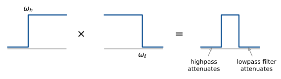
A highpass with cutoff omega_h times a lowpass with cutoff omega_l gives a bandpass. The highpass attenuates below the band and the lowpass filter attenuates above it.

Bandpass = cascade of lowpass and highpass, \omega_h < \omega_\ell

The only signals that pass are those that are in the passband of both filters.

To get a bandstop, we want the gain in the passband to be reasonably close to 1 (0 dB). Instead of cascading, where gains multiply, we use a parallel interconnection:

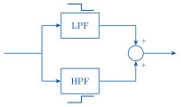
Parallel interconnection: the input feeds an LPF and an HPF, and their outputs are added at a summing junction.

The LPF passes low frequencies. The HPF passes high frequencies. Where their stopbands overlap, no signal passes.

Butterworth filters

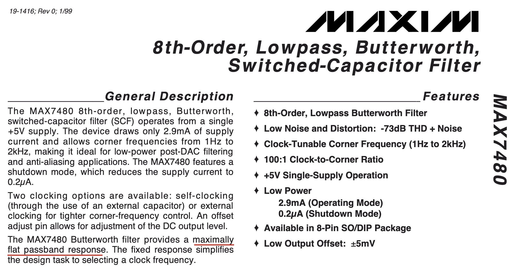
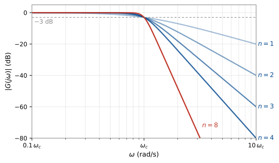
Header of the MAX7480 datasheet: 8th-order, lowpass, Butterworth, switched-capacitor filter, with the phrase maximally flat passband response underlined.

Butterworth filters are a popular practical filter design. The response is designed to have “maximally flat passband response”,¹ that is, no ripples in the gain response.

An n^{\text{th}} order lowpass Butterworth filter with cutoff frequency \omega_c is the stable filter with:

n poles
no zeros
magnitude response satisfies \lvert G(j\omega)\rvert^2 = \frac{1}{1 + \left(\dfrac{\omega}{\omega_c}\right)^{2n}}.

The gain is 1 at DC and \dfrac{1}{\sqrt{2}} (-3 dB) at \omega = \omega_c.

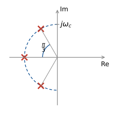
Butterworth gain in dB against omega for n = 1, 2, 3, 4 and 8. All pass through minus 3 dB at omega_c and fall at 20n dB per decade beyond it.

To get the desired magnitude response, we place n poles on the semicircle of radius \omega_c in the left half plane.

Three poles on the left half of the circle of radius omega_c, at angles 2 pi over 3, pi and 4 pi over 3, spaced pi over 3 apart.

Let’s see why this works:

\lvert G(j\omega)\rvert^2 = G(j\omega)\,G(-j\omega)

\text{so } G(s)G(-s) = \frac{1}{1 + \left(\dfrac{-s^2}{\omega_c^2}\right)^n}

(note if s = j\omega, -s^2 = \omega^2).

= \frac{\omega_c^{2n}}{\omega_c^{2n} + (-s^2)^n}.

So the poles of G(s)G(-s) are the roots of

\omega_c^{2n} + (-s^2)^n = 0.

1 + \left(\frac{-s^2}{\omega_c^2}\right)^n = 0.

Setting s = \omega_c e^{j\theta} (a point on the radius \omega_c circle), we have solutions at

\theta = \frac{(2k + 1)\pi}{2n} - \frac{\pi}{2}, \qquad k = 0, 1, \ldots, 2n - 1.

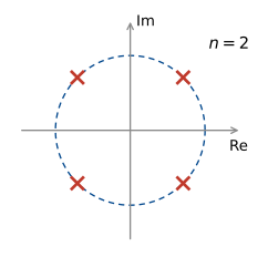
For n = 2, the four roots on the circle of radius omega_c at 45, 135, 225 and 315 degrees.

We then put all the left-half plane poles in G(s), then G(-s) has their reflections in the right half plane, so G(s)G(-s) has the right poles.

The first couple of Butterworth filters have the following transfer functions:

\begin{aligned} n = 1 &\qquad G(s) = \frac{\omega_c}{s + \omega_c} \\[12pt] n = 2 &\qquad G(s) = \frac{\omega_c^2}{s^2 + \sqrt{2}\,\omega_c s + \omega_c^2} \\[12pt] n = 3 &\qquad G(s) = \frac{\omega_c^3}{(s + \omega_c)(s^2 + \omega_c s + \omega_c^2)}. \end{aligned}

\left. \begin{aligned} n \text{ even} &\qquad G(s) = \prod_{k=1}^{n/2} \frac{\omega_c^2}{s^2 + 2\zeta_k\omega_c s + \omega_c^2} \\[12pt] n \text{ odd} &\qquad G(s) = \frac{\omega_c}{s + \omega_c}\prod_{k=1}^{(n-1)/2} \frac{\omega_c^2}{s^2 + 2\zeta_k\omega_c s + \omega_c^2} \end{aligned} \;\right\} \quad \zeta_k = \sin\!\left(\frac{(2k - 1)\pi}{2n}\right).

To get highpass filters, use the trick above: replace \dfrac{s}{\omega_c} with \dfrac{\omega_c}{s}.

Design example 2: heartrate measurement on a smartwatch

The heartrate monitor on a running watch or smartwatch uses photoplethysmography (PPG). An LED shines light into the wrist and a photodiode measures the reflection, which pulses with each heartbeat. A passband filter is used to remove both high and low frequency interference.

Passband: 30–240 bpm = 0.5 Hz to 4 Hz.

HF interference: mains power oscillates at 50 Hz, ambient light follows the square of the mains voltage at 100 Hz.

LF interference: breathing adds \approx 0.2 Hz oscillation.

For more info, have a look at this artice: how common noise and error sources affect optical biosensing.

To deal with these constraints, we have the following filter specification:

At most 3 dB loss at 0.5 Hz and 4 Hz.
At least 20 dB attenuation at 0.2 Hz.
At least 40 dB attenuation at 50 Hz.

Let’s draw these on a Bode diagram

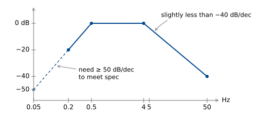
Specification on a Bode diagram: 0 dB from 0.5 Hz to 4 Hz, minus 20 dB at 0.2 Hz, minus 40 dB at 50 Hz. The low side needs at least 50 dB per decade, extended dashed to minus 50 dB at 0.05 Hz. The high side is slightly less than minus 40 dB per decade.

If we place Butterworth filters with \omega_h = 2\pi\times 0.5 rad/s, \omega_\ell = 2\pi\times 4 rad/s, we know we meet the -3 dB spec (this is the gain of a Butterworth at \omega_c).

We need n = 3 for the highpass and n = 2 for the lowpass.

\begin{aligned} n = 2 &\qquad G(s) = \frac{\omega_\ell^2}{s^2 + \sqrt{2}\,\omega_\ell s + \omega_\ell^2} \\[16pt] n = 3 &\qquad G(s) = \frac{\omega_h^3}{\left(\dfrac{\omega_h^2}{s} + \omega_h\right)\left(\left(\dfrac{\omega_h^2}{s}\right)^2 + \omega_h\left(\dfrac{\omega_h^2}{s}\right) + \omega_h^2\right)} \\[16pt] &\qquad\phantom{G(s)} = \frac{s^3}{(\omega_h + s)(\omega_h^2 + \omega_h s + s^2)} \end{aligned}

For a real example of a heart rate monitor filter, check out this chip: Analog Devices MAX30112

Footnotes

The largest possible number of derivatives of \lvert G(j\omega)\rvert^2 are zero at \omega = 0, without any transfer function zeros.↩︎